Image-to-Music-Playlist-Generator
Melodrip
Image to Music Playlist Generator
Authors: Pure and Saki
Link to Colab
Introduction:
April 20th, 2024 was Whitman College’s first hackathon. At this hackathon, Saki Bishop and Yuttanawee Buahom decided to participate as a two person team. At this hackathon, various ideas were put out but we were having a hard time settling on an idea, and thus were quite stumped as to what we should do. As we were racking our brains to find something unique and interesting to do, we found various models on huggingface that turns images into text and also classified lyrics into a music genre. Considering how fun it can be to play around with image generators, we were curious if we could combine the ideas of image to text and text to genre/mood to create a music playlist for a submitted image. The idea is that we would input a photo, which would then be given a caption that would next be analyzed into a theme, and then finally be grouped together with other songs of similar themes. With the usage of models from huggingface, we figured it could be possible to easily implement this despite there being many moving parts in this program. With these hackathon roots in mind, we have named this program after our hackathon team name, melodrip, coming from the imagery of new songs dripping upon us through recommendation.
Literature Review:
To get started on this project, we took a look at a YouTube video by Rithesh Sreenivasan titled “Text Summarization TextRank Algo Explain, spaCy pytextrank and genism python example #nlp“ , and also started reading on Cosine Similarity from a stackoverflow forum. Both of us were not too familiar with algorithms utilizing caption generation, and so the YouTube video was helpful in illuminating how text summarization works and how it is implemented through PageRank and TextRank. According to the video, there are two types of text summarization, extractive text summarization and abstractive text summarization. Extractive text summarization selects important sentences from a document to form a summary, and is grammatically correct but hard to read. Abstractive text summarization builds a semantic representation of the document, and utilizes paraphrasing techniques and at times adds original content to the summary. As we were planning on comparing generated captions with lyrics, it felt essential to focus on algorithms with extractive strategies rather than allowing the algorithm to add things that did not exist in either texts. PageRank had a focus on extracting information from website pages, and thus we settled on utilizing TextRank instead. As for the stackoverflow forum, we learned that the Scikit Learn library has a simple and easily implementable cosine metric. But to compare documents represented by keywords, it is important to have vector representations of the documents. It brings attention to TF-IDF vectorization, which was a concept we were more familiar with thanks to our Applied Machine Learning course.
Data Collection and Preprocessing:
The main data collection and preprocessing done for this project revolves around taking CSVs of song titles and lyrics, and then applying text normalization methods to make more accurate correlations. We also did the same preprocessing on the captions created by our image to caption generator. Our text normalization was first tokenizing the words, getting rid of any stop words or punctuation, and then stemming words that could be stemmed. Originally, as this project started off for the hackathon, we started the project using Taylor Swift’s discography as we were able to find a nice compilation of her songs by shaynak on github. This CSV contained the title, the album name, and the lyrics. When we were using this CSV, we took out the album information as it isn’t essential for our project. We first got rid of brackets that indicated certain sections such as [Chorus] and [Pre-chorus]. Next we applied our normalization method described above. As we worked with this CSV however, we realized that the 256 songs compiled was not enough to make any meaningful connections. Instead, we found a Kaggle dataset that contained a million songs from Spotify. This dataset contains the song title, artist name, lyrics, and links to the song. We hoped that we could utilize the links in the CSV to help direct our users to the songs directly, but the links did not always direct us to a Spotify link. Thus, we decided to get rid of the link section and get back to figure out a playlist creation algorithm at a later time. Next, because our normalization function did not work for the lyrics, we decided to just do some basic preprocessing of getting rid of ‘\n’ and ‘ ‘.
Methodology:
Our project largely dealt with transfer learning for the caption generator, the TextRank algorithm, TF-IDF vectorization, and cosine similarity. We also used StreamLit to create the user interface. First, the model used for the image captioning was BLIP-2 from Hugging Face. Proposed by Junnan LI, Dongxu Li, Silvio Savarese, and Steven Hoi, BLIP-2 is “a generic and efficient pre-training strategy that bootstraps vision-language pre-training from off-the-shelf frozen pre-trained image encoders and frozen large language models”. We had a couple other image captioning models that we worked with, but BLIP-2 had the most sentences that made sense, and thus BLIP-2 was chosen as the model to utilize in our project. The second algorithm we dealt with was TextRank. TextRank is a graph-based ranking model for text processing, used to extract the most relevant sentences or words. The graph in question takes key words as nodes, and the connections between each word as weighted edges. With this graph, TextRank assigns scores for each node depending on how many neighbors (or how many edges) it has. After TextRank was established, we were able to extract the top keywords by sorting the words by their score using lambda and turning the top 5 words into a list. TF-IDF vectorization was mainly used to match the extracted keywords from the caption and match it to the lyrics of the song. TF-IDf vectorizer compares the frequency of a word in a document with the number of documents the word appears in and assigns a measure of originality. We applied the TF-IDF vectorizer on all of the lyrics and turned it into a lyrics matrix. We also applied another TF-IDF vectorizer specifically on the extract keywords from the TextRank algorithm. Finally, we looked to find the similarity between the extracted keywords and lyrics matrix using cosine similarity. Cosine similarity is an algorithm that compares the angles of two vectors to measure how close the vectors are pointing to the same direction. With establishing similarity scores, we sorted the similarity scores so that we can extract the top 5 songs as our recommended songs. This project was our first time dealing with Sreamlit, but it was relatively simple. After importing the Streamlit app into Google Colab, we created a simple user interface in our main function. With guidance from a medium article by Yash Kavaiya, we were able to successfully run the interface through creating a local tunnel, and establishing a tunnel password by putting in our IP address.
Experimental Setup:
Our experimental set up consisted of testing the models over and over again with one photo, and printing out the results to see if it would make sense as a person logically. For the first round of testing we focused on a picture of a dog that is wearing sunglasses and licking its face (Figure 1). This will also be the example we will be showing in the results section.

For the image captioning section, we ran the picture through around 4 different image captioning algorithms that were available to us on Hugging Face. After selecting the caption that made the most sense and captured the essential parts of the image (i.e. a caption that says “a dog wearing sunglasses and a collar” makes more sense than “a dog sitting in front of a white background”), we moved to testing the keyword extraction process. This also consisted of printing the keywords and adjusting how weight is assigned depending on what keywords were being printed out. Finally, to make sure that the song recommendation algorithm made sense, we had some code that would print the lyrics and the similarity score so that we could compare the extracted keywords and lyrics side by side.
Results:
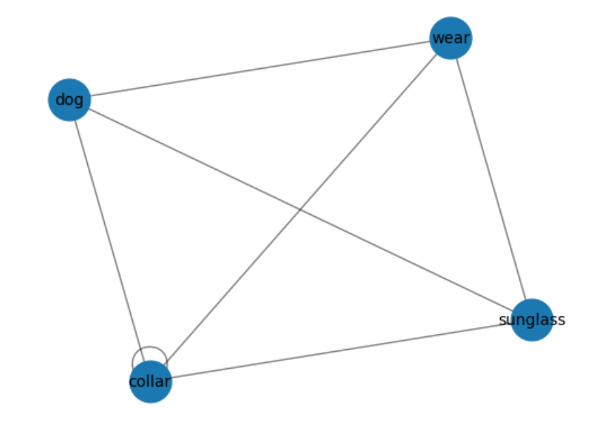
Ultimately, we were able to create a fun recommending system that takes in an image and compares the automatically generated image caption with various lyrics to recommend a song. As we have mentioned briefly, we will be focusing on the test image to display our results. For the picture of the white dog with funky sunglasses that is licking itself, the generated caption was “there is a dog wearing sunglasses and a collar with a collar”. After going through the preprocessing, TextRank, and keyword extraction functions, the key words were deemed as ‘collar’, ‘dog’, ‘wear’, ‘sunglass’. The following is a visualization of the graph that was fed into the buildGraph function (figure 2).
The next graph is the table showing the assigned TextRank score and the keywords (figure 3).

The TextRank visualization shows that all words have the same score except for collar, which we have noticed appeared twice in the image captioning. When compared with the lyrics matrix created with the TF-IDF vectorization, most songs that showed up were dog related as most of these songs would contain the words ‘dog’ and ‘collar’. The following table is the visualization of the 10 songs with the highest similarity scores (figure 4).
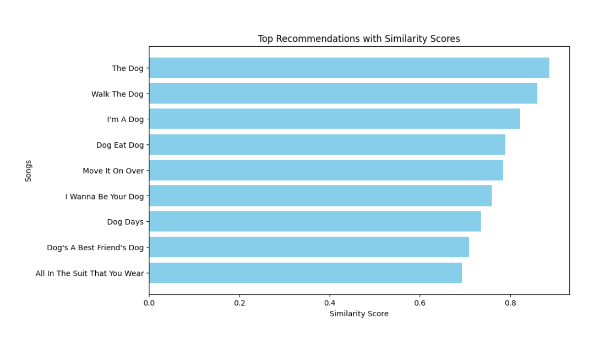
As we can see, even with the seemingly absurd photo of a dog, it was possible to find songs with similarity scores around 0.8, which is quite high. We kept the recommended songs within 5 songs, as the scores started to go under the similarity score of 0.8. For the songs that were recommended for this photo, it consisted of “The Dog” by Otis Redding at a score of about 0.8869, “Walk the Dog” by Eddie Cochran at about 0.8604, “I’m a Dog” by Gucci Mane at about 0.8218, “Dog Ear Dog” by Weird Al Yankovic at about 0.7891, and “Move It On Over” by Hank Williams at about 0.7847. Here is another instance of a photo running through this project. We have the following photo of a hammock on a palm tree on a beach side at sunset (figure 5). The caption given for this photo was “a close up of a hammock hanging from a palm tree on a beach”. When it was run through the keyword extractor, the keywords were ‘close’, ‘hammock’, ‘palm’, and ‘tree’. As each of these words showed up once, the TextRank scores were equal for each key word and thus the figures for the graph and TextRank visualization will be omitted. Figure 6 shows the top 10 recommended songs based off of the similarity scores.

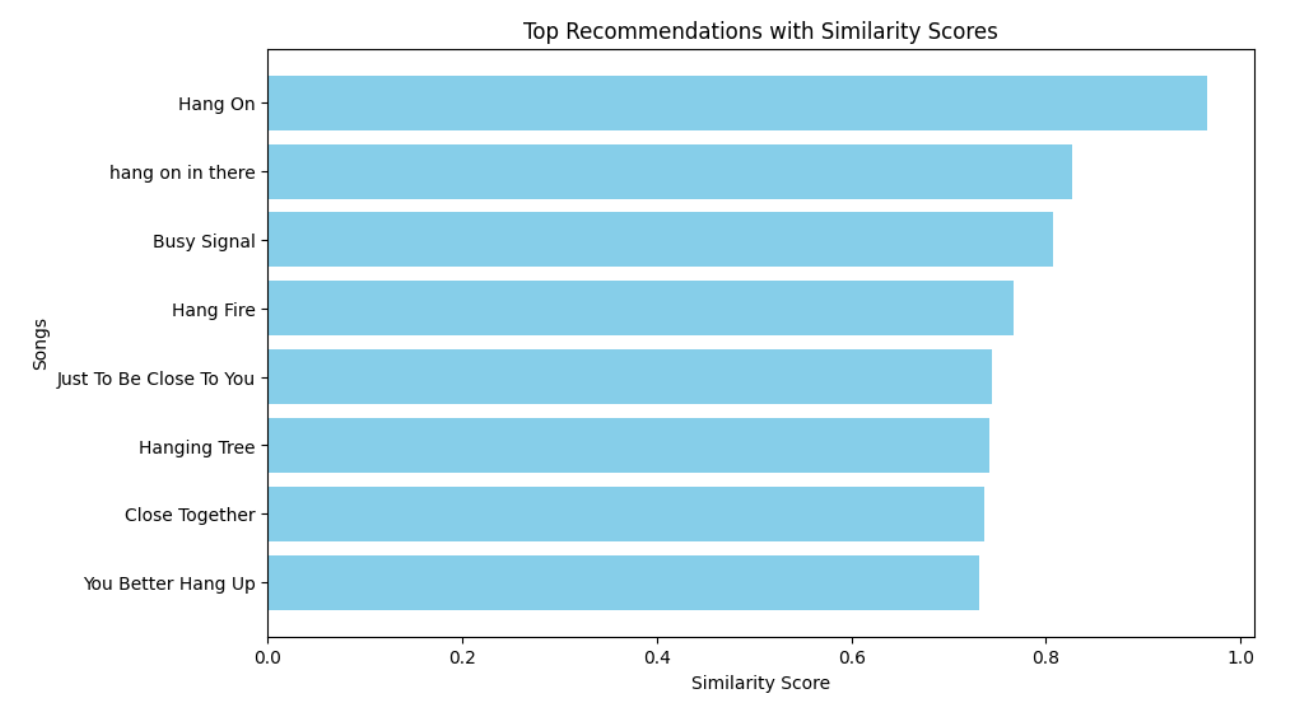
The songs that were recommended for the second photo consisted of “Hang On” by Weezer at a score of about 0.9664, “hang on in there” by John Legend at about 0.8269, “Busy Signal” by Dolly Parton at about 0.8070, “Hang Fire” by the Rolling Stones at about 0.7669, and “Hang On” by Michael W. Smith at about 0.7609. Again, we can see the decrease in similarity scores in around 5 songs, so 5 songs seemed the best number to recommend to our users.
Discussion:
Our project became something that is very fun to play around with. Not all of the songs recommended could be considered as highly accurate considering that scores tend to go down within 5 songs. This is largely due to the limiting quality of automated caption generators and the amount of song data that was fed into the project. Our results were highly reliant on the number of unique words used in the caption generated by the submitted image. This meant that there is a good amount of overfitting between the key words and song lyrics, which had led to the similarity scores dropping under 0.8 within the first 5 songs. We attempted to improve this by looking for an image captioning model that provided longer sentences. However, the typical usage of image captioning expects the model to provide concise explanations, and thus most of the image captioning models found provided very precise and short image descriptions. Feeding the generated caption into another elaborative caption model poses the possibility of adding things unrelated to the image, and thus we were restricted to the shorter but accurate image captioning models. Another contribution to this limit would be the amount of songs fed into the project. As we were coding on Google Colab, the million songs provided from the Kaggle CSV was quite large and used up a lot of the RAM of our computers. However, if we were to add even more songs and lyrics, and were to push this project through a computer with more processing space, we would be able to increase the similarity scores further. Spotify had over 100 million songs on their platform. If more of these songs could be used in our project, we will be able to produce higher similarity rates as there are more unique words for the project to analyze.
Conclusion and Future Scope:
In the end, through the creation of an image to music playlist generator, we have learned alot about TextRank, vectorization, and cosine similarity. In the future, as mentioned in the section above, we would be interested in utilizing a database with even more songs to improve on our similarity scores. There is also some interest in creating a caption generator that focuses on accuracy and detail over accuracy and conciseness, so that the project has more varied weight in the keywords and ultimately connects to a more precise similarity rate. While it was not discussed as much in this report, we are also interested in making the user interface more enjoyable for the user. Currently, it is quite blank and also does not have an easy way to access the songs. Our next goal is to make it more colorful and also find a way to create a playlist that the user could press and listen to on the spot.
References:
“About Spotify.” Spotify, April 23, 2024. https://newsroom.spotify.com/company-info/.
ellen, and scipilot. “Cosine Similarity between Keywords.” Stack Overflow, December 13, 2018. https://stackoverflow.com/questions/53753614/cosine-similarity-between-keywords. Kavaiya, Yash. “How to Run STREAMLIT Code in Google Colab.” Medium, November 11, 2023. https://medium.com/@yash.kavaiya3/running-streamlit-code-in-google-colab-involves-a-few-steps-c43ea0e8c0d9.
Li, Junnan, Dongxu Li, Silvio Savarese, and Steven Hoi. “BLIP-2.” Hugging Face, January 30, 2023. https://huggingface.co/docs/transformers/main/model_doc/blip-2. Mahajan, Shrirang. “Spotify Million Song Dataset.” Kaggle, November 21, 2022. https://www.kaggle.com/datasets/notshrirang/spotify-million-song-dataset/discussion.
Shaynak. “Taylor-Swift-Lyrics/Songs.Csv at Main · Shaynak/Taylor-Swift-Lyrics.” GitHub, April 2024. https://github.com/shaynak/taylor-swift-lyrics/blob/main/songs.csv.
Sreenivasan, Rithesh. “Text Summarization TextRank Algo Explained , Spacy Pytextrank and Genism Python Example #NLP.” YouTube, October 30, 2020. https://www.youtube.com/watch?v=qtLk2x59Va8.